The State of Rural

An economic and demographic update of rural Minnesota

June 2020

By Kelly Asche, Research Associate & Marnie Werner, Vice President, Research

For a printable version of the report, click here.

Each year, the Center for Rural Policy and Development provides a brief update on various economic and demographic data pertaining to rural Minnesota. As policy discussions concerning rural Minnesota unfold, it is important to understand the past, present, and potential futures of rural regions. This report provides historical data points that illustrate how rural conditions have changed and where they are at now, making for healthy discussions about the current demographic and economic vitality of these areas.

Rural Atlas Online

To supplement and support the annual State of Rural Minnesota report, we also maintain and regularly update an online, interactive collection of maps and charts that show readers this data broken down in different ways. In addition to this report with its high-level analysis, our Atlas of Minnesota Online provides more interactive maps and charts showing a variety of data on demographics, the economy and more at the state, county, planning region, and economic development region levels. To visit the site, click here.

A marker in time

As we review the new data for this year’s State of Rural report, it’s clear that this data will not accurately represent our current situation. Due to its recency, the COVID-19 pandemic and the subsequent changes in employment will not be reflected in the following data, and therefore, the following information should be thought of as a “marker in time,” a benchmark from just before the pandemic struck, which we can then compare to new data as they are released throughout this year and next.

 

Summary

People

Currently, population growth in Greater Minnesota is concentrated in larger metropolitan-designated counties such as Blue Earth, Stearns and Olmsted, the north central counties of Itasca, Cass and Hubbard, and in counties where there is a concentration of non-white populations, such as Kandiyohi and Mower.

Meanwhile, the most urban areas of the state, including the Twin Cities, have seen a significant increase in annual population gains compared to the previous decade, primarily due to a significantly larger international migration into these areas. Micropolitan cities in Greater Minnesota are expected to see continued growth as well but at a lower rate. Without growth in domestic or international in-migration in rural areas, most of rural Minnesota is projected to continue losing population over the next 20 to 30 years.

One aspect of these trends that continues to get overlooked, however, is the in-migration of 30- to 49-year-olds across Greater Minnesota. Many rural development organizations are recognizing this trend and are developing initiatives that focus on recruitment and retention in this age group.

Economic Vitality

There are few significant differences in employment when comparing urban and rural areas. Education and health services along with trade, transportation, and utilities employ nearly 50% of the labor force in most of our counties no matter how rural. Rural counties, however, have a higher percentage of people employed in agriculture and government jobs or are self-employed, while the Twin Cities area has a significant share of people employed in the professional and business services sector such as management of companies, legal advice and representation and accounting.

There continues to be significant opportunity for employment in regions outside of the seven-county metro. The highest job vacancy rates and largest increases in wages for job vacancies have occurred in Greater Minnesota.

Although the largest gains in earnings per job have occurred outside of the most urban counties, the growth hasn’t been enough to close the wage gap between these rural regions and the rest of the state. The agriculture sector experienced enormous growth in earnings between 2008 and 2012, but low earnings over the last four years have erased those gains.

Agriculture

Although agricultural land values are beginning to decline from their peak in 2014, they continue to be historically high, with land along the western side of the state holding its value the best. Meanwhile, low commodity prices and increases in the costs of production have created a situation where many farmers have a negative net income. Even when including government payments, which typically represent 2% to 3% of total farm income, most farmers are barely getting by.

 

Rural-Urban Commuting Area regions

Everyone has their own idea and definition of “rural” based on their perceptions—one person’s small town is another person’s weekend city shopping hub. However, anyone traveling across our state can agree that most of Minnesota can’t be categorized as strictly rural or metropolitan. Most places are in between.

To develop a better understanding of trends across Minnesota, this report displays data in two different way: a) maps highlighting data at the individual county level, and b) county-level data aggregated into four categories developed by the Minnesota State Demographer: entirely rural; town/rural mix; urban/town/rural mix; and entirely urban (Figure 1). As the names suggest, counties have been grouped based on the degree of their “ruralness” or “urbanness.” The appendix provides more complete definitions for each of these categories.

The number of counties within each category are: a) entirely rural: 14; b) town/rural mix: 35; c) urban/town/rural mix: 25; and d) entirely urban: 13.

Figure 1: The MN State Demographic Center analyzed census tracts in each county to determine their degree of “ruralness” or “urbanness.” Data: MN State Demographic Center

 

People

While the state’s most rural counties are still experiencing annual population declines, the rest of the state is seeing growth slowing. The exception is in entirely urban counties, which since 2010 have seen a significant increase in annual population gains. Meanwhile, although Minnesota has experienced an average annual net loss in domestic migration, urban counties have overcome that loss through significantly higher international migration.

Population gains slowing throughout Greater Minnesota while the most rural areas see declines continuing

Outside of the seven-county Twin Cities area, population growth can be found in three types of counties: counties that are considered recreational (central lakes), counties where non-white populations are concentrated (e.g. Nobles), and in metropolitan counties such as Blue Earth and Olmsted.

Figure 2: Population gains outside of the seven-county metro are in “recreational” counties and where non-white populations are concentrated. Data: U.S. Census Decennial Census & American Community Survey 5-year

 

Our most rural counties are the most likely to experience population loss, with an average of nearly 4% loss across the region. Of the 14 counties in the entirely rural group, only three saw population gains since 2010. The chances of a county experiencing population growth increases as the number of town and urban census tracts in that county increases (Table 1).

 

Table 1: Broken out by RUCA county groups, our most rural counties are least likely to experience population gains. Data: U.S. Census – Decennial Census & Population Estimates

RUCA county group	Counties in group	Counties with pop growth	% of counties with pop growth
Entirely rural	14	3	21%
Town/rural mix	35	17	49%
Urban/town/rural mix	25	18	72%
Entirely urban	13	12	92%

 

These population trends are driven by migration patterns, and the age, ethnicity and race of the population in rural Minnesota.

International migration and natural change driving changes in population growth rates.

A relatively significant change in Greater Minnesota’s population is occurring across the state, but that change varies depending on how rural or urban a county is. As Figure 3 shows, the more urban a county is, the more likely it is to have seen continued population growth, but between 2010 and 2019, that growth has slowed compared to the decade 2000-2010. The exception is in entirely urban counties, where growth in the current decade has continued to accelerate. The state’s most rural counties, however, have continued to see population loss on average, but the rate of loss has lessened so far this decade.

Figure 3: The town/rural and urban/town/rural mix county groups saw significantly lower annual population gains from 2010 to 2019 than they did from 2000 to 2010. Data: U.S. Census Bureau, Population Estimates

 

In counties with urban areas, the two primary variables that allow them to experience continued population growth rates is international migration and more births than deaths.

A significant difference in any of the rural county groups compared to the most urban areas is the lack of international migration. All regions are experiencing an annual net loss in domestic migration, or in the case of our entirely urban areas, minor gains. Our entirely urban areas, however, have been experiencing significant in-migration of populations from outside of the United States, whereas our more rural areas do not experience the same (Figure 4).

Figure 4: Although all regions have experienced either minor gains or more significant losses in domestic migration, counties that have more urban areas overcome this with significant gains through international migration. Data: U.S. Census Bureau, Population Estimates

 

The other significant difference between rural counties and counties with more urban areas is their ability to overcome outmigration with natural change. Natural change is the net gain or loss from the number of births and deaths. Without international migration, natural change can barely make up for out-migration from our more rural counties. Counties in the entirely rural group, in fact, continue to see more deaths than births, meaning those counties are experiencing on average both outmigration and negative natural change (Figure 5).

Figure 5: Natural change can barely overcome outmigration in counties with a town/rural mix, whereas more urban counties experience more births than deaths and an in-migration. Entirely rural areas experience an overall outmigration and more deaths than births (negative natural change). Data: U.S. Census Bureau, Population Estimates

 

Population gains partially driven by race and ethnicity

In Greater Minnesota, nonwhite and Latino populations tend to be concentrated in a few areas, such as St. Cloud, Worthington, and Rochester, while the demographics in the rest of the region have stayed largely unchanged. The counties where these populations are concentrated in Greater Minnesota are typically the same locations that are currently experiencing population gains. This becomes more evident in the southern half of Minnesota where much of the overall population decline is concentrated except in counties with higher percentages of non-white or Latino populations (e.g., Nobles, Mower, Kandiyohi).

 

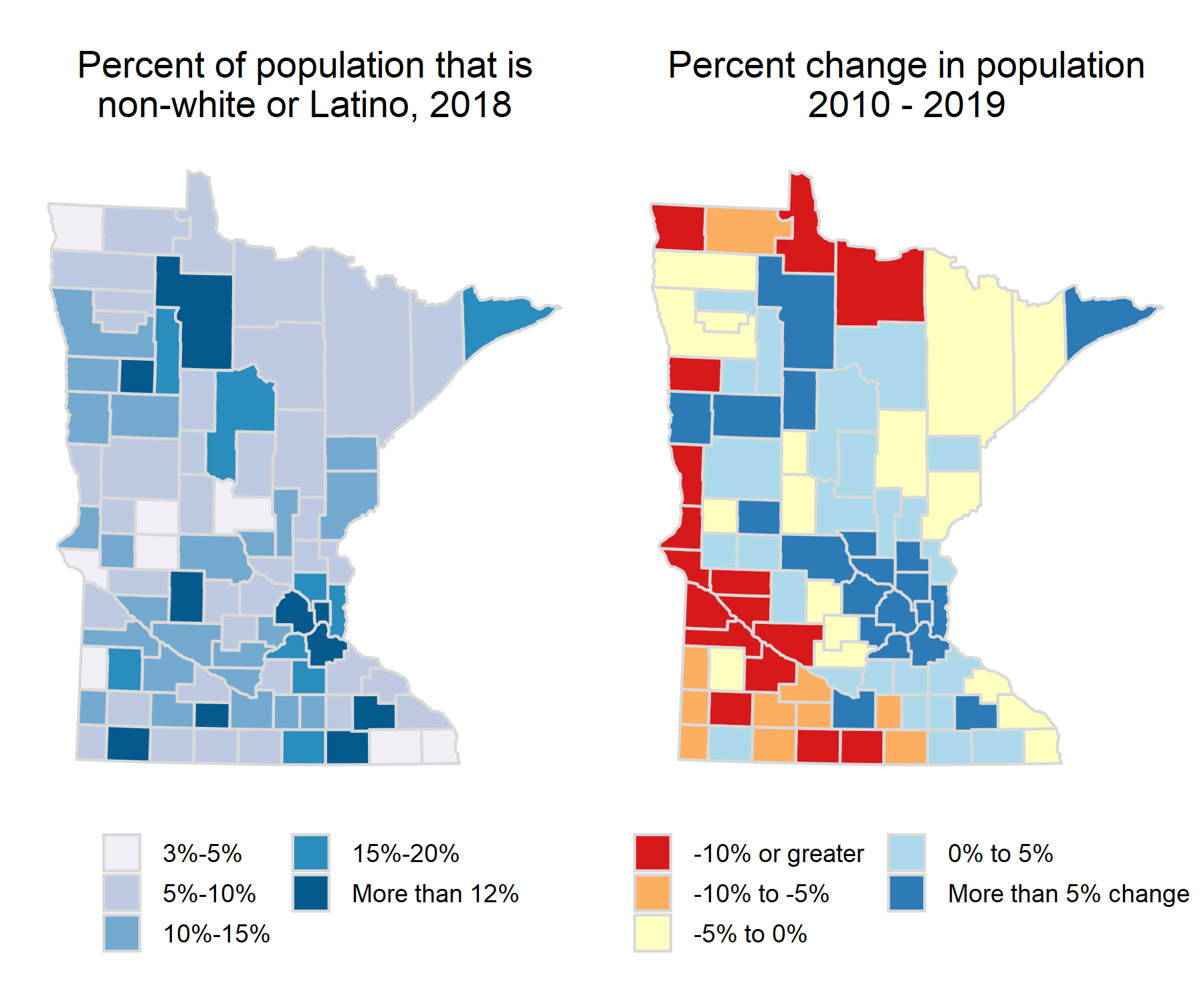
Figure 6: Non-white and Latino populations typically make up a larger percentage of the population in southern Minnesota than in northern counties.  The counties with the highest percentages typically have experienced overall gains in their population as well. Data: U.S. Census Bureau, Decennial Census & Population Estimates

 

People recruitment: in-migration of 30- to 49-year-olds

One aspect of migration data that can be hidden is the trend in migration by age group. Even though most rural areas have been experiencing an overall out-migration, it is not always a loss among all age groups. In fact, many rural counties see an in-migration of people between the ages of 30 and 49. In lakes regions, that age range extends out to include even older households as they retire and move to lake homes.

Many rural development organizations, county boards, and municipal organizations are participating in “people recruitment” strategies to take advantage of this migration pattern, which is well documented by University of Minnesota Extension[1]and in our report on recruiting workforce.

Figures 9 and 10 provide a glimpse into this trend. For any location in the state, it can be expected that if all conditions stay the same, the number of 25- to 29-year-olds counted in the 2010 census will be equal to the number of 15- to 19-year-olds counted in the 2000 census—the same people, just ten years older. All conditions do not stay the same, however: at the end of that ten-year period there may be more or fewer people than should be expected for that age group—hence an in-migration or out-migration.

Such is the case in Minnesota. Between 2000 and 2010, almost all rural counties experienced an out-migration of people who would be 25 to 29 years old in 2010 (Figure 7). They had migrated away somewhere in the previous ten years. But while this age group was migrating out, the next age group older, those entering their early 30s in 2010, were migrating into these rural counties. The question now, of course, is whether the 2020 Census will show this trend continuing.

 

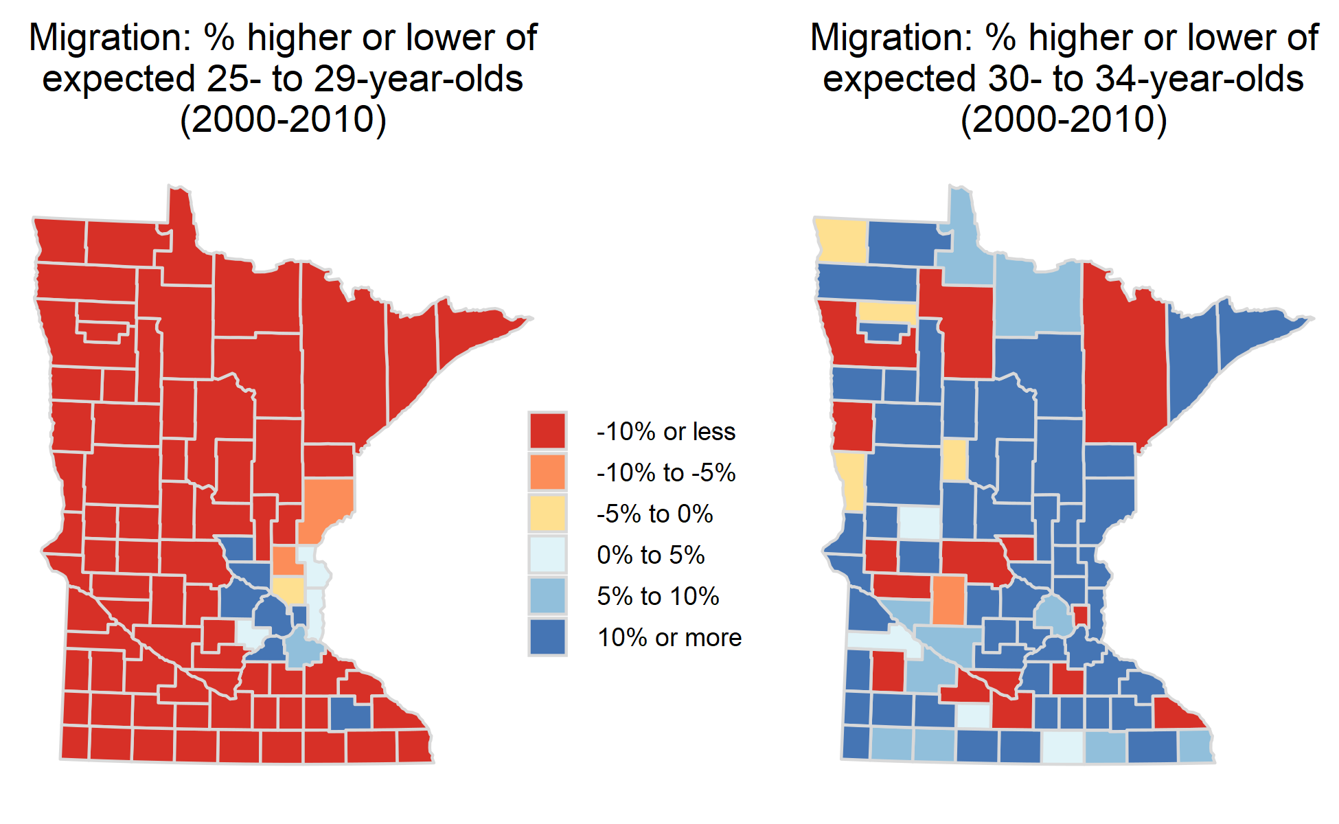
Figure 7: The percent change in the number of 25- to 29-year-olds between 2000 and 2010. All counties outside the Twin Cities area except Olmsted and Benton saw an out-migration of 25- to 29-year-olds. The percent change in the number of 30- to 34-year-olds between 2000 and 2010. Rural counties saw significant in-migration of 30- to 34-year-olds. Rural areas tend to see this trend up to 49-year-olds. Data: U.S Census Bureau Decennial Census

 

Economic vitality

Similar to the state’s urban areas, the rural economy is diverse, and while education and health services sector is the top employer in most counties, other industries, such as agriculture in western counties, are also significant. Greater Minnesota also has the highest job vacancy rates and the largest increases in wages for job vacancies.

Rural areas have a higher percentage employed in government, agriculture, and self-employment

One issue that arises when looking at jobs and employment in rural areas is that many data sources do not capture farm employment due to many of the workers not being covered by typical unemployment insurance programs. The information provided below is a mix of two data sources in an attempt to capture the employment impacts of agriculture. Although mixing two data sources can be problematic, we feel that this more accurately captures the worker-industry environment than just leaving out agriculture altogether. It should also be kept in mind that, as our report on the impact of agriculture on rural Minnesota’s economy shows, a large part of what we think of as agriculture—food processing, non-food processing, commodities trading—is in reality ag-related industry and is categorized into several separate industry sectors, including manufacturing, transportation, and financial.

The following map and tables provide the industries with the highest percentage of workers. The top employing industries are strikingly similar across all of Minnesota, although there are other top employment industries that match regions where we would expect. The highest percentage of employment continues to be in the education and health services industry sector across most of Minnesota. However, agriculture becomes more prominent in western counties, leisure and hospitality in a few northern counties, and manufacturing in central and southern Minnesota (Figure 8).

Figure 8: Education and health services is the dominant industry sector across Minnesota in terms of highest employment. Other industries take the top spot where expected, such as agriculture in western counties and leisure and hospitality in some northern counties. Data: Bureau of Labor Statistics, Quarterly Census of Employment and Wages; Bureau of Economic Analysis, Local Area Personal Income and Employment.

 

Top industries around the state in terms of employment include trade, transportation and utilities; leisure and hospitality; manufacturing; construction; farm employment; and professional and business services. The one significant difference between the regions is the high employment in the professional and business services in the entirely urban group of counties (Table 2). 

 

Table 2: Top five employment industries by planning region. Includes percent of total employment in each industry. Data: Bureau of Economic Analysis, Local Area Personal Income and Employment

Rank	Entirely rural	Town/rural mix	Urban/town/rural mix	Entirely urban
1	Education and Health  Services, 22.056%	Education and Health  Services, 23.752%	Education and Health  Services,  26.456%	Education and Health  Services,  24.932%
2	Farm employment, 18.395%	Trade, Transportation  and Utilities,  19.064%	Trade, Transportation  and Utilities,  18.558%	Trade, Transportation  and Utilities,  18.326%
3	Trade, Transportation  and Utilities, 17.686%	Manufacturing,  15.337%	Manufacturing,  13.814%	Professional and  Business Services,  15.681%
4	Leisure and  Hospitality, 11.971%	Leisure and  Hospitality,  9.066%	Leisure and  Hospitality,  9.872%	Leisure and  Hospitality,  9.922%
5	Public  Administration, 7.011%	Farm employment,  7.995%	Professional and  Business Services,  5.692%	Manufacturing,  9.646%

 

Another difference is in the percentage of people employed by government. Government is a major employer in many rural counties, where the need for a baseline of services can be disproportionate to the population. In 2017, 18% of total jobs in the entirely rural county group were in government, 14% in the town/rural group, 13% in the urban/town/rural group, and 10% in the entirely urban county groups, respectively (Figure 9). 

Figure 9: Government jobs include the executive, legislative, judicial, administrative and regulatory activities of federal, state, and local governments and the military, plus government enterprises, which are government agencies that cover a substantial portion of their operating costs by selling goods and services to the public. These types of jobs make up a significantly higher percentage of the jobs outside of the entirely urban areas. Data: Bureau of Economic Analysis, Regional Personal Income and Employment

 

Figure 10: The highest percentage of jobs in government is in northern and western Minnesota. Data: Bureau of Economic Analysis, Local Area Personal Income and Employment

 

It’s no surprise that farming is a significant source of employment for the more rural areas of the state. Western counties have the highest percentage of employment in agriculture, with many over 20%. The largest share is in Marshall County, where 32% of employment are in agriculture. However, in most southern Minnesota counties 10% or fewer of the jobs are in agriculture (Figure 11). 

Figure 11: Farm employment is the number of workers engaged in the direct production of agricultural commodities, either livestock or crops, whether as a sole proprietor, partner, or hired laborer. These workers as a percentage of employment typically make up 20% or more of total employment in counties dominated by agricultural. Data: Bureau of Economic Analysis, Local Region Personal Income and Employment & U.S. Census Bureau, ACS 5-year

 

Another notable characteristic of employment in rural regions is the number of non-employers and self-employed. The state’s most rural regions have a higher percentage of these entities in relation to total jobs compared to more urban regions (Figure 12). It’s particularly high in northern counties, where non-employers and self-employed can represent 12% to 18% of total jobs. The highest percentage is in Hubbard County with 18.2% (Figure 13). 

Figure 12: The percentage of the workforce recognized as operating non-employer businesses is significant in most rural areas of Minnesota. Being a non-employer means an individual operates a non-farm business with no employees, has annual business receipts of at least $1,000, and is subject to federal income tax. Data: Census Bureau, Non-Employer Statistics

 

Figure 13: The highest number of self-employed and non-employers as a percentage of total jobs are in northern Minnesota. Hubbard County has the highest percentage with 18.2%. Data: U.S. Census Bureau, Non-Employer Statistics

 

Gap in earnings continues to grow

“Average earnings by place of work” shows the wages workers make, as opposed to their income, which can include both earned income, such as wages, and unearned income, such as interest and dividends. “Jobs” includes both full-time and part-time jobs (but is not the same as “employment” or “workers,” since one worker can hold more than one job at a time) and includes wage and salary jobs, sole proprietorships, and individual general partnerships, but not unpaid family workers or volunteers. This measure can be especially useful when assessing the economic vitality of areas in Greater Minnesota since it takes into account farm and non-employer incomes that are not captured in many other economic measurements.

Figure 14 shows that the gap in average earnings between the entirely urban county group and the other three county groups continues to increase. In the entirely rural county group, earnings experienced a significant increase between 2011 and 2013, largely due to the sharp rise in farm incomes, but that growth has dropped off considerably since then.

Currently, average earnings in the entirely rural county group are 61% of average earnings for the state, while average earnings in the town/rural group and the urban/town/rural mixed group are 71% and 77% respectively.

Figure 14: Earnings per job shows an increasing gap between entirely urban counties and the rest of the state. Agricultural income can have a significant impact on entirely rural counties, which can be seen between 2008 and 2014. Data: Bureau of Economic Analysis, Regional Personal Income and Employment

 

Figure 15: Earnings per job is significantly higher in the seven-county metro area while moderately high earnings are scattered throughout Greater Minnesota. Counties in southern Minnesota typically have higher earnings per job than counties in northern Minnesota. Data: Bureau of Economic Analysis, Local Area Personal Income and Employment

 

Despite this continued gap, though, the highest growth in earnings per job since 2001 continues to be in rural regions. In 2017, the earnings per job in the entirely rural group was $38,728, which is 59% higher than in 2001, the largest gain out of all the county groups. The town/rural mix, urban/town/rural mix and entirely urban county groups saw gains of 57%, 55% and 49% over 2001 levels respectively (Figure 16).

Figure 16: Despite the increasing gap in earnings per job between rural and urban areas, increases in earnings among rural counties were significantly higher during the recession, but have since dropped and kept pace with the larger metropolitan counties. Data: Bureau of Economic Analysis, Regional Personal Income and Employment

 

Greater Minnesota feeling pressure to fill job vacancies

Job vacancies are increasing across the state and are at their highest levels at any point since 2005. This increase is largely due to retirements in the workforce as well as continued economic growth.

To get a sense of the pressure a region might feel in filling these vacancies, Figure 17 provides the average quarterly number of job vacancies for each year as a percentage of total jobs in the region. The higher the percentage, the more challenging it is to fill the positions. The highest percentages exist in regions outside of the seven-county metro. Southwest Minnesota currently has the highest percentage, where the average quarterly number of vacancies in 2018 represented 6.3% of the total filled jobs in the region. 

Figure 17: The job vacancy rate is the ratio of vacant job positions to all jobs. A high vacancy rate indicates a relatively strong demand for workers. The highest job vacancy rates exist outside of the Twin Cities seven-county metro. Data: MN DEED Job Vacancy Survey

 

Although the median wages for all job vacancies continue to be lower in Greater Minnesota than in the seven-county metro area, the largest increases in wages have occurred in Greater Minnesota. In 2005, the median wage for job vacancies in Greater Minnesota ranged from $2.30 to $3.40 lower than in the seven-county Twin Cities area. By 2017, the gap had shrunk to $0.80 to $2.20 lower (Figure 18). 

Figure 18: The median wages of all job vacancies in regions outside the Twin Cities are increasing steadily. Data: MN DEED Job Vacancy Survey

 

Use of public assistance is greatest in the most rural areas

Social Security payments are made up of monthly payments to retired and disabled persons, their dependents and survivors, plus lump-sum payments to survivors. This does not include medical payments, however. The distribution of Social Security dollars from county to county is largely a reflection of the distribution of senior citizens. Therefore, we expect the highest per-capita payments to be in the most rural areas (Figure 19).

Figure 19: Not surprisingly, the largest social security payments are in counties with higher percentages of 65-year-olds or older. Data: Bureau of Economic Analysis Local Region Personal Income and Employment, U.S. Census Bureau ACS 5-year

 

Despite the highest per-capita payments in more rural regions, the largest growth in per-capita social security payments has been in more urban areas. Social security payments in entirely urban counties in 2001 averaged $1,231 but had grown to $2,770 by 2018, an increase of 125%. The other county groups saw increases of 110%, 107% and 92% in urban/town/rural mix, town/rural mix, and entirely rural groups, respectively. 

Public assistance payments include family assistance, food stamp payments, general assistance, supplemental security payments and other income maintenance benefits for families in need. It does not include medical payments or farm program payments.

The highest income maintenance benefits per capita continue to be in more rural areas. A few counties in northern Minnesota, where poverty rates tend to be higher, have some of the highest per-capita payments, exceeding an average of $1,000 per person (Figure 20). 

Figure 20: Public assistance payments include family assistance, food stamp payments, general assistance, supplemental security payments and other income maintenance benefits for families in need. It does not include medical payments or farm program payments. Data: Bureau of Economic Analysis, Local Region Personal Income and Employment & U.S. Census Bureau, ACS 5-year

 

Agriculture

After peaking in 2014, farmland values are beginning to decline. More importantly, net income for farmers also continues to decline due to low commodity prices and increases in the costs of production, leaving many farmers with a negative net income. (For more on this topic, see our report, “The Impact of Minnesota’s Farm Economy on Greater Minnesota.”)

Land values declining from 2014 peak but still historically high

Current land value estimates by the University of Minnesota Land Economics department remain historically high as they continue to reflect in part the high returns from farming between 2008 and 2012, and though they declined after that, the overall value per acre has plateaued over the last three years (Figure 21). In 2017, the value of ag land per acre for Minnesota was $4,804, down 3% from 2016. However, demand for farmland for residential and commercial development has also driven up values, as can be seen in the urban and suburban counties of the Twin Cities, where ag land values are the highest (Figure 22).

Figure 21: Farmland is defined as all agricultural 2a land, including Green Acres, minus the house/garage/first acre and the building site. This was called “deeded” land prior to 2009. The significant increase in value between 2011 and 2014 is due to the high returns from farming, while increasing pressure for residential and commercial development is keeping values up in and around metropolitan areas. Data: University of Minnesota Land Economics

 

Figure 22: The value of agricultural land is highest in the metropolitan areas due to increased pressure from commercial and residential development. Data: University of Minnesota Land Economics

 

The value of farmland increased dramatically between 2009 and 2014. Even in today’s poor ag economy, estimated farmland values in counties in the entirely rural group, where farmland dominates, were estimated to be 80% higher in 2017 compared to 2009, while in the entirely urban counties in Minnesota farmland was estimated to be 27% higher. The change in the value of farmland, however, varies greatly from county to county. In fact, farmland in Hennepin and Ramsey counties, the northern suburbs and counties stretching into the north-central lakes region has dropped in value since 2009. The largest increases have occurred in central and southern Minnesota (Figure 23).

Figure 23: Change in agricultural land values since 2009 shows considerable variation across the state. The largest increases have occurred in central and southern Minnesota. Data: University of Minnesota Land Economics

 

Net income for farming continues to decrease

The following chart shows the cost of production and cash receipts received per acre for farmers in Minnesota. These elements are defined as:

• Total cash receipts: gross revenue received by farmers from the sale of crops, livestock, and livestock products and of the value of defaulted loans made by Commodity Credit Corporation and secured by crops; and,
• Production expenses: purchases of feed, livestock and poultry, seed, fertilizer, agricultural chemicals and lime, and petroleum products; labor expenses; machinery rental and custom work; animal health costs; and all other expenses, including depreciation.

Starting in 2015 and continuing into 2018, the cost of production has equaled or exceeded the cash receipts for farmers in Minnesota due to natural increase in costs of inputs and low commodity prices. In 2018, the cost of production was $710 per acre while cash receipts were only $713 per acre (Figure 24).

Figure 24: Starting in 2015 and continuing through 2018, the overall cost of production has equaled or exceeded cash receipts for farms per acre. Data: Bureau of Economic Analysis, Local Region Personal Income and Employment

 

Federal government payments to farm operators consist of deficiency payments under price support programs for specific commodities, disaster payments, conservation payments, and direct payments to farmers under federal appropriations legislation.

The bulk of government payments in 2018 are attributable to agricultural commodity programs. In Minnesota, the median payment was 3.7% of total farm income. The largest percentages were in northwestern Minnesota, where percentages ranged from 4% to 14%. 

Figure 25: The bulk of government payments to farmers in 2018 are attributable to agricultural commodity programs. The average payments were 2.4% of total income across Minnesota. Data: Bureau of Economic Analysis, Local Region Personal Income and Employment

 

When including government payments, income still isn’t enough to cover the cost of production for many farmers. The highest net income for farms exists in the seven-county metro and in southwestern Minnesota (Figure 26).

Figure 26: Net income includes cash receipts from marketings, government subsidies, and other income while subtracting the cost of production. In a majority of Minnesota counties, farmers are making less than $50 per acre or losing money. Data: Bureau of Economic Analysis, Local Region Personal Income and Employment

 

Appendix: Rural-Urban Commuting Areas

Throughout this report we present information using four county groups developed by the State Demographer and Minnesota’s Demographic Center derived from the USDA’s Rural-Urban Commuting Area codes. This definition provides a handy way to look at counties by similar characteristics rather than location.

Staff at the Minnesota Demographic Center examined each Census tract in the state to determine its “type” using the definitions in the Rural-Urban Commuting Area framework (explained below). Each county was then classified by its “mix” of Census tracts. For example, if a county has one Census tract that can be defined as “small town” and all other Census tracts could be defined as rural, the county is categorized as “town/rural mix.” The number of counties within each category are i) entirely rural: 14; ii) town/rural mix: 35; iii) urban/town/rural mix: 25; and iv) entirely urban: 13.

Figure 27 shows how each county is categorized. 

Figure 27: These categorizations are based on an analysis of the rural-urban commuting areas at each county’s census tract level. Data: MN State Demographic Office

 

The United State Department of Agriculture Economic Research Service developed the Rural-Urban Commuting Area codes as a way to define geographic areas using more than population alone. These codes incorporate population density, urbanization, and daily commuting to define a geographic area. Below are the ten primary RUCA codes, grouped into their four geography definitions.

Urban Definition

1	Census tract is situated at the metropolitan area’s core and the primary commuting flow is within an urbanized area of 50,000 residents or more.
2	Census tract is within a metropolitan area and has higher primary commuting (30% or more) to an urbanized area of 50,000 residents or more.
3	Census tract is within a metropolitan area and has lower primary commuting (10-30%) to an urbanized area of 50,000 residents or more.

 

Large Town Definition

4	Census tract is situated at a micropolitan area’s core and the primary commuting flow is within a larger urban cluster of 10,000 to 49,999 residents.
5	Census tract is within a micropolitan area and has higher primary commuting (30% or more) to a larger urban cluster of 10,000 to 49,999 residents.
6	Census tract is within a micropolitan area and has lower primary commuting (10-30%) to a larger urban cluster of 10,000 to 49,999 residents.

 

Small Town Definition

7	Census tract has a primary commuting flow within a small urban cluster of 2,500 to 9,999 residents.
8	Census tract has higher primary commuting (30% or more) to a small urban cluster of 2,500 to 9,999 residents.
9	Census tract has lower primary commuting (10-30%) to a small urban cluster of 2,500 to 9,999 residents.

 

Rural Definition

10	Census tract has a primary commuting flow outside of urban areas and urban clusters.

 

The Minnesota State Demographer’s office analyzed each county to determine the combinations of census tract types in each one. The counties were then categorized into 4 groups:,

• Entirely rural: every census tract was rural;
• Town/rural mix: the county had at least one census tract that was rural, and small or large town census tracts;
• Urban/town/rural mix: the county had at least one census tract that was rural, small or large town, and urban; and,
• Entirely urban: every census tract was urban.

For more information about these definitions check out their report – “Greater Minnesota: Refined & Revisited”

Figure 28: Each census tract was given one of the four definitions from the table above. Data: MN State Demographic Office