

Marnie Werner, VP Research
Click here for a printable version of this report.
Between 2000 and 2015, the price of farmland in the United States climbed to record levels, driven first by high farm income derived from high demand for corn for use in biofuels,[1] then by high demand for any kind of reliable investment during the Great Recession. Between 2015 and 2020, ag incomes fell and land prices stayed fairly level, but by 2021, the farmland market was beginning to heat up again. During that year, the average price of farmland in Minnesota rose 10%, according to the USDA,[2] and 30% on average in Iowa, according to the Federal Reserve Bank of Chicago.[3]
At first glance, these record prices bring up memories of the land bubble that burst in the early 1980s ushering in the Farm Crisis. This time around, these record-high prices are still concerning, but for different reasons: high land prices are making it difficult for farmers with fewer resources—especially beginning farmers—to acquire more land; more land is being bought by individuals and even investment firms that don’t live in the area; and for local governments, which depend on local property taxes for revenue, these record-high selling prices are hyperinflating the ag land portion of their tax bases. As a result, in the state’s most active farming regions farmland now accounts for more than 75% of the tax base, according to Minnesota Department of Revenue data.
The high percentage of property value concentrated in one type of land raises concerns that local tax bases are too undiversified in these regions and that too much local government revenue is dependent on only one type of property. In the event of a crash in that property type’s value, local governments could take a serious hit to their revenue. In this analysis, we’ll look at how big a role ag land plays in the tax base in various regions of the state, what a decline in values could mean for property tax revenue, and the other problems this lack of diversification could be causing.
In very simplified terms, a local government’s tax base is the amount of property tax revenue the properties in that entity’s jurisdiction can generate after various exclusions and deductions have been applied but before state property taxes and local referendum property taxes have been added in. What properties are included can vary by taxing authority, but in general the tax base is equivalent to the local net tax capacity.[4] As a rule, property taxes make up about 40%–50% of a county government’s annual revenue. Other local governments that depend on property taxes include cities, townships, and school districts, plus smaller entities such as regional development commissions and county soil and water districts.
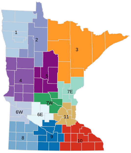
For property tax purposes, land is divided into several categories, or classifications, based on how it is being used. Since the Minnesota Department of Revenue uses 15 classifications overall, we grouped them into five larger categories: residential, agricultural, cabins (seasonal recreational property), commercial/industrial, and “other” (including apartments, utilities, railroads, personal property, and other miscellaneous types). All property tax data is from the MN Department of Revenue unless otherwise noted. For this project we compared individual economic development regions, or EDRs, each region containing five to ten counties.
Undiversified: Tax bases differ region to region
Diversification in a tax base is a good thing: it means that at any one time, a government is deriving its revenue from more than one source—preferably several different sources. Diversification lowers risk by spreading it around. The growth in the price of farmland has been so strong, however, it is causing farmland valuations to dominate local government tax bases, especially in Minnesota’s most agricultural regions.
The forces driving farmland prices have traditionally been based on the land’s productivity, measured by how much revenue it can generate from the products it produces (corn, wheat, beef, etc.).[5] This was especially true between 2000 and 2008, when an average acre of Minnesota farmland more than doubled in value, from about $1,280 to $2,700.[6] This link to productivity also shows in the way the rise in farmland prices hasn’t been consistent around the state. More-productive farmland in far western, southwestern, and southern Minnesota gained more value compared to farmland in less ag-focused regions (Figure 1).
Figure 1: Minnesota’s most productive farmland regions have seen the most growth in farmland value while the rest of their tax bases have stayed steady or grown more slowly.
Every region has its own unique mix of property types, and that mix can vary quite a bit region to region and county to county. Which property type dominates depends on location. For example, EDRs 6W and 8 in the southwest corner of the state take in some of Minnesota’s most productive farmland. In 2021, farmland made up 69% of EDR 8’s tax base and 77% of EDR 6W’s (Figure 2).
Figure 2: Farmland in economic development regions 6W and 8 makes up a significant share of the regions’ tax bases.
Other EDRs are more diversified, not because they’re doing anything better but because more of the land in those locations is better suited for non-ag purposes. EDR 5’s tax base reflects its location in the central lakes region of north central Minnesota: it is dominated by residential properties (38%) and cabins (31%) with a smaller amount of agricultural property (13%) thrown in (Figure 3). In EDR 4, the tax base is divided evenly between agriculture and residential property (31% and 35% respectively), with the other one third divided among commercial/industrial, cabins, and “other.”
Figure 3: EDRs 4 and 5 have more diversified tax bases where two or more types of property dominate.
Compared to EDRs 4 and 5, 6W and 8 look quite undiversified, but so does one other region: EDR 11, the seven-county Twin Cities region. Here, residential property made up nearly 60% of the region’s tax base in 2021, while commercial/industrial represented another 27% and “other,” another 13% (Figure 4).
Figure 4: In the seven-county Twin Cities region, residential property value makes up a majority the tax base, with commercial and industrial properties comprising another quarter.
While reliance on one property type for the local tax base is not inherently bad, as mentioned earlier, it adds risk. When the Great Recession struck in 2009 causing home prices to plummet nationwide, the residential portion of EDR 11’s tax base contracted, going from a peak of $2.5 billion in net tax capacity to $1.85 billion in 2014, a decline of 24%. At the same time, the commercial/industrial segment of the tax base lost $150 million, shrinking by about 14%. The two sectors’ losses had a definite effect: the entire tax base contracted by 18% over those five years.
During that time, though, regions like EDR 6W and EDR 8 saw little effect. While the market for housing contracted, the agricultural economy, and therefore the market for ag land, barely paused.
Table 1: Regional net tax capacity by property type. The Great Recession affected regional tax bases differently depending on which type of property made up more of the tax base.
“When we had the Great Recession, things were just chugging along here,” says Jake Sieg, who now serves as Lac Qui Parle County administrator after fifteen years as county auditor. Lac Qui Parle County is in EDR 6W, and at its peak in 2015, ag land there made up 90% of the county’s tax base; in 2021, it was 85%.
“If you weren’t reading a newspaper, you had no idea that there was a recession in the rest of the country, because that’s exactly when farms were doing better than they ever have since I’ve been here,” Sieg said.
During the recession, farmland looked like the only stable investment left, which drew more non-farmer investors seeking a safe place for their dollars into the market. Then, when farm incomes eventually tumbled beginning in 2014, farmland values should have tumbled as well based on the rule that land value is tied to income. But instead, land values only stalled, hovering around a statewide average of just under $5,000 an acre between 2015 and 2020.
Land prices adjusted after 2014, “but it wasn’t a crash,” says Kent Thiesse, Senior Vice President in ag lending at MinnStar Bank in Lake Crystal, MN, and a long-time University of Minnesota Extension agent.
By the time the Great Recession arrived, land prices were already becoming detached from farm income. A 2014 study of farmland in several agricultural states found that, depending on where the farmland was located, other factors were now playing into demand: “agricultural returns alone do a poor job of describing farmland values.”[7] The potential for land development, in fact, turned out to be “… a significant determinant of market value,” accounting for as much as half the market value for farmland located near population centers.[8]
The risks of another crash
So, what does it mean for local governments if the value of ag land has become disconnected from the usual drivers, and does it portend another bubble bursting?
Probably not, says Thiesse. Today’s economic situation is very different from the 1970s, which makes a repeat of that crash unlikely. Here’s why.
• Low interest rates. Perhaps the biggest threat to farmland prices is a rise in interest rates, but that is also the biggest difference between now and fifty years ago: interest rates are much lower today, says Dr. William Lazarus, a professor and Extension economist in the Applied Economics department at the University of Minnesota. In the 1970s, the U.S. economy was struggling under high inflation and high unemployment—“stagflation”—but at the same time farmland values were being driven upward, partly by high commodity prices and partly by loans being offered to farmers for 95% of the value of the land. Because of these loans, farmers had very little equity in their land, so when the Federal Reserve raised interest rates drastically in 1981 in an effort to tame inflation, new loans became very expensive, the demand for land dried up, and the value of farmland plummeted.
Figure 5: Farm real estate loan interest rates have been dropping steadily since the 1980s.
Since the 1980s, interest rates have been dropping steadily, which has been driving much of the demand for ag land since 2000. Lower interest rates reduce the cost of debt, which means if land prices fall, buyers won’t be as crippled by their debt load. At the same time, says Thiesse, farmers buying land today are buying with more cash—50% or more. This lower debt-to-asset ratio leaves borrowers in a safer position if farmland values drop.
Even though the Federal Reserve has announced a plan to slow inflation in 2022 by raising interest rates, the increases are expected to be small and measured. Land prices may fall, but not by much and not too drastically, says Thiesse.
• Tax-favored options help drive demand. Helping to push demand for land is the 1031 exchange, a tax-deferral tool in the IRS code that wasn’t around in the 1980s. The 1031 exchange allows investors to defer the capital gains taxes resulting from the sale of an investment by buying the same type of investment. Farmers hold land for decades, and therefore, when they decide to sell, the capital gains taxes that sale triggers can be substantial. Using a 1031 exchange, farmers—and real estate investors in general—are able to sell their land, then purchase essentially the same type of land, preferably in an area where it’s less expensive, allowing them to buy more of it, all while deferring their capital gains taxes. Showing up at a land auction with a large amount of money from their land sale does make farmers more competitive, says Thiesse.
• Today’s government programs and profitability. The federal government has created an array of programs over the years designed to keep farmers afloat in difficult times, but in the last ten years especially, those programs have proliferated.
For rural, ag-dependent counties, land value is still more attached to ag profitability than, say, potential development. But even when farm incomes plunged after 2013 (Figure 6),[9] land values stayed relatively stable in rural areas, and federal farm programs have a great deal to do with that, says Megan Roberts, recently an educator in the Agricultural Business Management division of the University of Minnesota Extension and now executive director of the Minnesota State Southern Agriculture Center of Excellence. In the last few years, the federal government has moved beyond regular Farm Bill Title I programs and Title XI crop insurance programs to create additional ad-hoc programs, says Roberts, like the Market Facilitation Program, which addressed the impact of the Chinese embargo on American farm products, and the Coronavirus Food Assistance Program. These programs have helped ensure that farm operators could continue to make mortgage payments or pay their rent, despite lower commodity prices, Roberts says.
Figure 6: Farm earnings can be quite volatile. Government payment programs intended to keep farmers afloat have also contributed to keeping farmland profitable over the last ten years.
Fertilizer prices started shooting up in 2021 and are expected to double in 2022, according to Lazarus. Farmland prices, however, kept going up, driven by continued low interest rates and improved farm income, even though the federal government started phasing out the CFAP program toward the end of the year.[10] Still, a major change in farm programs when farm incomes are low could threaten the farmland market if profitability goes away.
• A word on today’s inflation and the Russia-Ukraine war. A new wrinkle, however, is the Russian invasion of Ukraine. Oil prices have spiked since the conflict began in late February, which could have an impact on farm profitability, but grain prices have spiked also. Both Russia and Ukraine are major grain suppliers on the world market. According to Kansas State University, the conflict “will cause major disruptions in the world wheat market and significant disruptions in the world corn market.”[11] Even without government payments, Lazarus’s calculations project that farm income should be just fine this upcoming year, but that projection is “of course, very dependent on the crop prices,” he said. Since real estate has traditionally been the hedge against inflation for investors, “oil increases and the global uncertainty just continue to speak to higher inflation and higher volatility,” says Roberts, which could help land prices up, not hurt them. “Only time will tell for certain, though.”
Other potential problems
• Any drop in land values could be an issue for revenues because of the way tax rates are structured. Like residential property, ag land can also be homesteaded, qualifying the land for a a more favorable tax rate (Table 2).[12]
Table 2: Different classifications of farmland are taxed at different rates.
In ag-heavy counties, the vast bulk of land value is 2a agricultural homesteaded and non-homesteaded land. (Class 2a agricultural homestead HGA property (house, garage & first acre) has little impact on the tax base in most counties.) The tiered tax rate applied to homesteaded ag land makes a difference when the value of ag land changes. The example in table xx shows how, if the taxable land value of a piece of property were to drop by a third, from $3 million to $2 million, the tax revenue on a homesteaded piece of property would drop by one half (49%), not one third as it does with non-homesteaded land.
Table 3: If the value of ag land were to fall, the hit to property tax revenues would be different based on whether the land was classified as homesteaded or non-homesteaded.
• Little margin for error. Although a drop of that size is unlikely, even a small decrease in overall ag land values could still cause problems for property-tax payers in a county like Lac Qui Parle.
The issue, says Lac Qui Parle’s county administrator Sieg, is not so much that farmland values might go down, but that, if they did, there isn’t much of a cushion. The other property classes besides agriculture in our most rural counties—residential, commercial/industrial, railroad, utilities, and others—are growing slowly (Table x), but their overall share of the tax base is shrinking (Figure x). Between 2005 and 2019, the overall tax base of EDR 6W, of which Lac Qui Parle County is a part, nearly tripled, growing 198%. The commercial/industrial and cabin tax bases more than doubled, growing 122% and 123% respectively. The residential tax base, however, grew only 30% in those 15 years, and agricultural homestead HGA only grew 8%. The drivers in tax base growth were, of course, agricultural homesteaded and agricultural non-homestead, which together more than quadrupled in value (325%). In 2005, farmland represented 59% of the total tax base of EDR 6W; by 2019 it made up 78%.
At the same time, county levies keep growing little by little each year, says Sieg, which means that in a county like Lac Qui Parle, with a small, aging population, the increase in the ag land tax base is basically sheltering other taxpayers from these increases in levies.
Table 4: In EDR 6W, ag land far outstripped other categories in terms of growth in value and was responsible for almost 90% of the region’s growth in tax base.
• The continued rise in prices can make counties appear “wealthy.” High ag land values also have an impact on state aid to counties, school districts, and other local jurisdictions. While property taxes make up about half of local government revenue, state aid fills in most of the other half, about 40%–50%. The state’s complex formulas for calculating aid to local governments include calculating the ratio of tax base to population. If that ratio grows—more “wealth” per capita—it’s perceived as a good thing and that the local government needs less help in the form of state funding. That might be the case in a county with a large population and a large diversified tax base, but in Swift County, where ag land made up 75% of the county’s tax base in 2019, that’s a problem.
“Because of the lower population of the county [estimated at 9,359 in 2019], higher ag value isn’t a benefit,” says Swift County administrator Kelsey Baker. “Lower ag values would provide more benefit for county program aid benefit.” Swift County’s tax base per capita in 2019 was $2,706. In comparison, Hennepin County’s ratio was $1,689, while Stearns County’s was $985. Lac Qui Parle County’s ratio was $2,836. When these ratios were plugged into the state’s County Program Aid formula, funding to these “high-wealth” counties dropped.
This high tax-base-per-capita ratio in counties with small populations had created a false picture of a county’s ability to generate revenue locally, making it appear wealthier than it actually was. Table 2 shows the result if ag land is removed from the tax-base-per-capita equation: Swift and Lac Qui Parle suddenly look much more in line with counties where ag doesn’t play as big a role.
Table 5: The ratio of tax base per capita can be used to indicate a county’s property wealth in comparison to other counties, but for counties rich in ag land and sparse in population, it indicates a more complicated situation.
The fact that a large part of the tax base value is owned by an even smaller set of taxpayers complicates the situation further. Currently, Swift County has 5,237 separate taxpayer numbers on its property tax rolls. Of those, 2,105 own agricultural land, which means 40% of the taxpayers are responsible for at least 75% of the county’s tax base.
Many rural school districts face a similar problem: the potential tax pressure on a few landowners has often made it difficult to pass levy referendums for school funding in rural areas, says Sam Walseth, government affairs director for the Minnesota Rural Education Association. School districts can raise funding locally to supplement funding from the state through either an operating levy referendum for operating funds or a bond levy referendum for capital improvements such as a new school building or repairs on an old building, but both types of funding must for the most part be approved by district voters.
In terms of bonding, all ag land is included when calculating the bonding levy, which until recently meant bonding referendums in ag-heavy school districts often failed. “The farm community has been upset about the price tag that they pay,” says Walseth. “When they’re out there, and they’re representing 60% or 70% of the property, and the voters are basically asking—or the school is asking—them to pay 50%, 60%, 70% of a $50 million mortgage—if you’re one of ten or twenty-five families, how do you feel about that?”
In the case of operating funds, farmers and other farmland owners aren’t generally the impediment to passing a referendum since farmland is excluded from an operating fund levy except for agriculture homestead HGA, which tends to represent a small portion of the overall agriculture tax base in rural districts.
Because they can’t include the much higher-value homesteaded and non-homesteaded ag land in operating levies, rural school districts are “in a way impoverished … because we can’t tax one of our biggest resources, which is agricultural land,” says Walseth.
In all three of these situations—counties, school bonding referendums, and school operating referendums—the legislature has addressed the issues using different tools.
- For counties, legislators adjusted the tax-base equalization portion of the formula that determines state aid to counties to include a multiplier that increases per-resident funding for counties with small populations. The change recognized that the rapid rise in farmland values was inflating tax bases and distorting the true picture of finances in many rural counties.[13]
- In 2017, school districts, ag groups, the Minnesota Rural Education Association, and legislators worked together to create the Ag2School tax program to address the difficulty of passing bonding referendums. In its first year, the state provided a 40% property tax credit to farmland owners on bonding levies. The credit will eventually scale up to 70% in 2023.[14] At least one study has shown an increase in successful bonding referendums in rural districts since Ag2School was passed.[15] While naysayers worry that the program will disappear, Walseth calls it a big win for rural school districts and the rural economy.
- To ease the difficulty school districts were having passing operating referendums, legislators agreed to allow school boards to levy $724 per pupil without a referendum. This property tax increase, if the school board chooses to enact it, falls only on the non-ag property taxpayers in the district, which represent a small percentage of the total tax base in ag-heavy districts.
Looking ahead
The unique situation of Minnesota’s western, southwestern, and southern counties created local government revenue problems that the rest of the state does not often experience: a tax base largely dependent on one type of property. Fortunately, stakeholders were able to work with legislators in the last few years to find remedies to the most obvious problems.
But the growth in ag land prices is not over yet. The Swift County assessor informed the board of commissioners in mid-March that his office increased the estimated market value on tillable ag land in the county by 20%, a $400 million increase. The county’s estimated market value must be between 90% and 105% of average sales prices of that property type; Swift County’s value came in at 92%. What does that mean? It means that that county assessor’s per-acre estimated market value came in on the low end of the average sales price scale, suggesting that the price of ag land is not slowing down.
This land boom is being driven by a unique time in history that has created a unique set of factors: an already hot market, a massive amount of liquid cash introduced into the economy in the last two years, and a war in Europe driving a lot of uncertainty. The first of the Federal Reserve’s eight planned interest rate hikes happened March 16, so we will see what impact those have on the market, but so many farmers and other investors are paying in cash, even an increase in interest rates may not slow things down.
What this means for policymakers is the likelihood of more problems for rural local governments—like the “county wealth” formula—that they, and even local government officials, can’t anticipate.
One thing is known, however: the market for agricultural products plays out on a global stage and changes day to day. That’s important, not just for the farmers’ incomes but also for the overall economy of Minnesota, which still derives a good portion of its revenue from the agricultural sector. And while the rise in ag land values may not pose an immediate threat to county revenues, diversification of the rural tax base in agricultural counties should remain a goal. The risk of placing too much trust in an undiversified tax base has ramifications right down to the least populated counties, cities, and school districts.
[1] Key, Nigel. “Financial Conditions in the U.S. Agriculture Sector: Historical Comparisons,” U.S. Department of Agriculture, Economic Research Service, 2019, 8. https://www.ers.usda.gov/webdocs/publications/95238/eib-211.pdf
[2] U.S. Department of Agriculture, “USDA QuickStats.” https://quickstats.nass.usda.gov
[3] Oppedahl, David, “AgLetter,” Federal Reserve Bank of Chicago, February 2022. https://www.chicagofed.org/publications/agletter/2020-2024/february-2022
[4] MN Department of Revenue, “Glossary.” https://www.revenue.state.mn.us/glossary-t
[5] Henderson, Jason, “Will Farmland Values Keep Booming?” Economic Review, vol. 93, issue 2, 2008.
[6] USDA QuickStats. https://quickstats.nass.usda.gov
[7] Borchers, Allison, et al., “Linking the Price of Agricultural Land to Use Values and Amenities,” American Journal of Agricultural Economics, vol. 96, issue 5, 2014.
[8] Ibid.
[9] Although still in line with the 1970-2020 average, according to USDA’s Economic Research Service.
[10] Federal Reserve Bank of Chicago, “AgLetter,” 1/3/22. https://www.chicagofed.org/research/data/ag-conditions/index
[11] Briggeman, Brian C., “Ukraine and Russian Conflict—Understanding Macroeconomic Effects,” 2022 Risk and Profit Online Mini-Conference: “Ukraine–Russia Conflict—Agricultural Ramifications,” Kansas State University, Agricultural Economics, March 7, 2022. https://agmanager.info/2022-risk-and-profit-online-mini-conference-presentations/ukraine-and-russian-conflict-understanding
[12] Minnesota Department of Revenue, “Minnesota Property Tax Administrator’s Manual,” 2021. https://www.revenue.state.mn.us/property-tax-administrators-manual
[13] Minnesota House Research, “County Program Aid,” February 2020. https://www.house.leg.state.mn.us/hrd/pubs/ss/sscpa.pdf
[14] Sieg, Jake. “Minnesota’s Ag2School Property Tax Credit,” Lac qui Parle County Auditor-Treasurer, July 24, 2019. https://www.lqpv.org/docs/district/documents/minnesota%27s%20ag2school%20property%20tax%20credit%20-%20july%2024,%202019.pdf?id=1083
[15] Jensen, Sheldon. “Land of 10,000 Schools? An analysis of Minnesota’s Ag2School tax credit program,” 2021.